Home
Bibliography
Contact
Interesting Articles
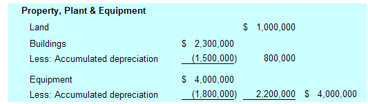
Items of property, plant, and equipment are included in a separate category on a classified balance sheet. Property, plant, and equipment typically follows the Long-term Investments section, and is oftentimes simply referred to as "PP&E." Items appropriately included in this section of the balance sheet are the physical assets deployed in the productive operation of the business, like land, buildings, and equipment. Note that idle facilities or land held for speculation may more appropriately be listed in some other category on the balance sheet (like long-term investments) since these items are not in productive use. Within the PP&E section, the custom is to list PP&E according to expected life -- meaning that land (with an indefinite life) comes first, followed by buildings, then equipment. For some businesses, the amount of PP&E can be substantial. This is the case for firms that have heavy manufacturing operations or significant real estate holdings. Other businesses, say those that are service or intellectual based, may actually have very little to show within this balance sheet category. At right is an example of how a typical PP&E section of the balance sheet might appear. In the alternative, some companies may relegate this level of detailed disclosure into a note accompanying the financial statements, and instead just report a single number for "property, plant, and equipment, net of accumulated depreciation" on the face of the balance sheet.
COST TO ASSIGN TO ITEMS OF PROPERTY, PLANT, AND EQUIPMENT: The correct amount of cost to allocate to PP&E is based on a fairly straight-forward rule -- to identify those expenditures which are ordinary and necessary to get the item in place and in condition for its intended use. Such amounts include the purchase price (less any negotiated discounts), permits, freight, ordinary installation, initial setup/calibration/programming, and other normal costs associated with getting the item ready to use. These costs are termed "capital expenditures." In contrast, other expenditures may arise which were not "ordinary and necessary," or benefit only the immediate period. These costs should be expensed as incurred. An example is repair of abnormal damage caused during installation of equipment.
To illustrate, assume that Pechlat Corporation purchased a new lathe. The lathe had a list price of $90,000, but Pechlat negotiated a 10% discount. In addition, Pechlat agreed to pay freight and installation of $5,000. During installation, the lathe's spindle was bent and had to be replaced for $2,000. The journal entry to record this transaction is:
| 03-17-X4 |
Equipment |
86,000 |
||
|
Repair Expense |
2,000 |
|||
| Cash |
88,000 |
|||
| Paid for equipment (($90,000 X .90) + $5,000), and repair cost |
INTEREST COST: Amounts paid to finance the purchase of property, plant, and equipment are expensed. An exception is interest incurred on funds borrowed to finance construction of plant and equipment. Such interest related to the period of time during which active construction is ongoing is capitalized. Interest capitalization rules are quite complex, and are typically covered in detail in intermediate accounting courses.
TRAINING COSTS: The acquisition of new machinery is oftentimes accompanied by employee training regarding the correct operating procedures for the device. The normal rule is that training costs are expensed. The logic here is that the training attaches to the employee not the machine, and the employee is not owned by the company. On rare occasion, justification for capitalization of very specialized training costs (where the training is company specific and benefits many periods) is made, but this is the exception rather than the rule.
A DISTINCTION BETWEEN LAND AND LAND IMPROVEMENTS: When acquiring land, certain costs are again ordinary and necessary and should be assigned to Land. These costs obviously will include the cost of the land, plus title fees, legal fees, survey costs, and zoning fees. But other more exotic costs come into play and should be added to the Land account; the list can grow long. For example, costs to grade and drain land to get it ready for construction can be construed as part of the land cost. Likewise, the cost to raze an old structure from the land may be added to the land account (net of any salvage value that may be extracted from the likes of old bricks or steel, etc.). All of these costs may be considered to be ordinary and necessary costs to get the land ready for its intended use. However, at some point, the costs shift to another category -- "land improvements." Land Improvements is another item of PP&E and includes the cost of parking lots, sidewalks, landscaping, irrigation systems, and similar expenditures. Why do you suppose it is important to separate land and land improvement costs? The answer to this question will become clear when we consider depreciation issues. As you will soon see, land is considered to have an indefinite life and is not depreciated. Alternatively, you know that parking lots, irrigation systems, etc. do wear out and must therefore be depreciated.
LUMP-SUM ACQUISITIONS: A company may buy an existing manufacturing facility, complete with land, buildings, and equipment. The negotiated price is usually a "turnkey" deal for all the components. While the lump-sum purchase price for the package of assets is readily determinable, assigning costs to the individual components can become problematic. Yet, for accounting purposes, it is necessary to allocate the total purchase price to the individual assets acquired. This requires a pro-rata allocation of the purchase price to the individual components. This concept is best illustrated with an example:
Suppose Dibitanzl Corporation acquired a manufacturing facility from Malloy Corporation for the grand total of $2,000,000. To keep it simple, we will assume that the facility consisted of land, building, and equipment. If Dibitanzl had acquired the land separately, it is estimated that its fair value would be $500,000. The fair value of the building, by itself, is estimated to be $750,000. Finally, the equipment would cost $1,250,000 if purchased independent of the "package" deal. The accounting task is to allocate the cost of $2,000,000 to the three separate pieces. If you sum the perceived values of the components, you will note that it comes to $2,500,000 ($500,000 + $750,000 + $1,250,000). Yet, the actual purchase price was only 80% of this amount:
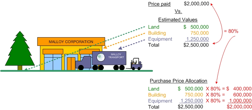
The above calculations form the basis for the following entry:
| 05-12-X7 |
Land |
400,000 |
||
|
Building |
600,000 |
|||
|
Equipment |
1,000,000 |
|||
| Cash |
2,000,000 |
|||
| Purchased land, building, and equipment |
EQUIPMENT LEASES
Many businesses acquire needed assets via a lease arrangement. With a lease arrangement, the lessee pays money to the lessor for the right to use an asset for a stated period of time. In a strict legal context, the lessor remains the owner of the property. However, the accounting for such transactions looks through the legal form, and is instead based upon the economic substance of the agreement.
If a lease effectively transfers the "risks and rewards" of ownership to the lessee, then the applicable accounting rules dictate that the lessee account for the leased asset as though it has been purchased. The lessee records the leased asset as an item of property, plant, and equipment, which is then depreciated over its useful life to the lessee. The lessee must also record a liability reflecting the obligation to make continuing payments under the lease agreement, similar to the accounting for a note payable. Such transactions are termed "capital leases." You should note that the basic accounting outcome is as though the lease agreement represents the purchase of an asset, with a corresponding obligation to pay it off over time (the same basic approach as if the asset were purchased on credit).
Of course, not all leases effectively transfer the risks and rewards of ownership to the lessee. The determination of risk/reward transfer is based upon evaluation of very specific criteria: (1) ownership transfer of the asset by the end of the lease term, (2) minimum lease payments with a discounted present value that is 90% or more of the fair value of the asset, (3) a lease term that is at least 75% of the life of the asset, or (4) some bargain purchase element that kicks in before the end of the lease. If a lease does not include at least one of the preceding conditions, it is deemed not to be a "capital lease," and is thus considered to be an "operating lease." You will be relieved to know that you have already studied "operating leases" in the earliest chapters of this book -- that is, rent is simply recorded as rent expense as incurred -- the underlying asset is not reported on the books of the lessee.
Your life's experiences may give you a basis for extending your understanding of leases. If you have rented an apartment at some point in your life, consider how it would be accounted for by you -- as a capital lease or an operating lease? None of the "4" criteria was likely met; thus, your agreement was an operating lease. In the alternative, you may have leased a car. It is possible (not assured) that your lease agreement would trigger one of the four criteria. If you were to follow generally accepted accounting principles for such an agreement, you would have recorded both an asset (the car) and the liability (obligation under capital lease) on your books the day you drove away from the dealer (in debit/credit context, you debit the asset and credit the liability for an amount that approximates the fair value -- I'll leave those details for intermediate accounting courses).
Now, you may wonder why all the trouble over lease accounting? However, if you think about an industry that relies heavily on capital lease agreements, like the commercial airlines, you can quickly come to see the importance of reporting the planes and the fixed commitment to pay for them. To exclude them would render the financial statements not representative of the true nature of the business operation.
SERVICE LIFE AND COST ALLOCATION
DEPRECIATION: Casually, people will speak of depreciation as a decline in value or using-up of an asset. However, in accounting jargon, the term is meant to refer to the allocation of an asset's cost to the accounting periods benefited -- not an attempt to value the asset. Thus, it is often said that depreciation is a process of "allocation" not "valuation." We have already addressed how an asset's cost is determined. Next, we must consider how to determine the accounting periods benefited (i.e., "service life").
Determining the service life of an asset is an essential first step in calculating the amount of depreciation attributable to a specific period. Several factors must be considered:
Physical deterioration -- "Wear and tear" will eventually cause most assets to simply wear out and become useless. Thus, physical deterioration serves to establish an outer limit on the service life of an asset.
Obsolescence -- The shortening of service life due to technological advances that cause an asset to become out of date and less desirable.
Inadequacy -- An economic determinant of service life which is relevant when an asset is no longer fast enough or large enough to fill the competitive and productive needs of a company.
Factors such as the above must be considered in determining the service life of a particular asset. In some cases, all three factors must be considered. In other cases, one factor alone may control the determination of service life. Importantly, you should observe that service life can be completely different from physical life. For example, how many computers have you owned, and why did you replace an old one? In all likelihood, its service life to you had been exhausted even though it was still physically functional.
Recognize that some assets have an indefinite (or permanent) life. One prominent example is land. Accordingly, it is not considered to be a depreciable asset.
DEPRECIATION METHODOLOGY
After the cost and service life of an asset are determined, it is time to move on to the choice of depreciation method. The depreciation method is simply the pattern by which the cost is allocated to each of the periods involved in the service life. You may be surprised to learn that there are many methods from which to choose. Four popular methods are: (1) straight-line, (2) units-of-output, (3) double-declining-balance, and (4) sum-of-the-years'-digits.
Before considering the specifics of these methods, you may wonder why so many choices. Perhaps a basic illustration will help address this concern. Let us begin by assuming that a $100 asset is to be depreciated over 4 years. Under one method, which happens to be the straight-line approach, depreciation expense is simply $25 per year (shown in red below). This may seem very logical -- especially if the asset is used more or less uniformly over the 4 year period. But, what if maintenance costs (shown in blue) are also considered? As an asset ages, it is not uncommon for maintenance costs to expand. Let's assume the first year maintenance is $10, and rises by $10 each year as follows:
STRAIGHT-LINE
DEPRECIATION PATTERN (red) and MAINTENANCE COSTS (blue):
Combining the two costs together reveals an interesting picture, showing that total cost rises over time, even though the usage is deemed to be constant.
COMBINED
COSTS:
The following graphics show what happens if we run the same scenario with an alternative depreciation method called sum-of-the-years'-digits (the mechanics will be covered shortly):
SUM-OF-THE-YEARS'
DIGITS DEPRECIATION PATTERN (red) and MAINTENANCE COSTS (blue):

COMBINED
COSTS:

Now, the combined cost is level, matching the unit's usage/cost and perceived benefit to the company. Arguably, then, the sum-of-the-years' digits approach achieves a better matching of total costs and benefits in this particular scenario. Does this mean that sum-of-the-years' digits is better? Certainly not! The point is simply to show an example that brings into focus why there are alternative depreciation methods from which to choose. In any given scenario, ample professional judgment must be applied in selecting the specific depreciation method to apply. The above discussion is but one simple illustration; life affords an almost infinite number of scenarios, and accountants must weigh many variables as they zero-in on their preferred choice under a given set of facts and circumstances (author's note: Not meaning to detract from the importance of this discussion, it must be noted that the choice of depreciation method can become highly subjective. Some research suggests that such choices are unavoidably "arbitrary," despite the best of intentions). Having set the stage for consideration of multiple depreciation methods, it is now time to dig into the mechanics of each approach.
MANY METHODS: A variety of approaches can be used to calculate depreciation. And, those methods are usually covered in intermediate accounting courses. Fortunately, most companies elect to stay with one of the fairly basic techniques -- as they all produce the same "final outcome" over the life of an asset, and that outcome is allocating the depreciable cost of the asset to the asset's service life. Therefore, although you will now only be exposed to four methods, those methods are the ones you are most apt to encounter.
SOME IMPORTANT TERMINOLOGY: In any discipline, precision is enhanced by adopting terminology that has very specific meaning. Accounting for PP&E is no exception. An exact understanding of the following terms is paramount:
- Cost: The dollar amount assigned to a particular asset; usually the ordinary and necessary amount expended to get an asset in place and in condition for its intended use.
- Service life: The useful life of an asset to an enterprise, usually relating to the anticipated period of productive use of the item.
- Salvage value: Also called residual value; is the amount expected to be realized at the end of an asset's service life. For example, you may anticipate using a vehicle for three years and then selling it. The anticipated sales amount at the end of the service life is the salvage or residual value.
- Depreciable base: The cost minus the salvage value. Depreciable base is the amount of cost that will be allocated to the service life.
- Book value: Also called net book value; refers to the balance sheet amount at a point in time that reveals the cost minus the amount of accumulated depreciation (book value has other meanings when used in other contexts -- so this definition is limited to its use in the context of PP&E).
Below is a diagram relating these terms to the financial statement presentation for a building:

In the above illustration -- assuming straight-line depreciation -- can you determine the asset's age?
It is 15 years old; the $2,000,0000 depreciable base ($2,300,000 - $300,000) is being evenly spread over 20 years. This produces annual depreciation of $100,000. As a result, the accumulated depreciation is $1,500,000 (15 X $100,000).
THE STRAIGHT LINE METHOD
Under this simple and popular approach, the annual depreciation is calculated by dividing the depreciable base by the service life. An asset that has a $100,000 cost, $10,000 salvage value, and a four-year life would produce the following amounts:
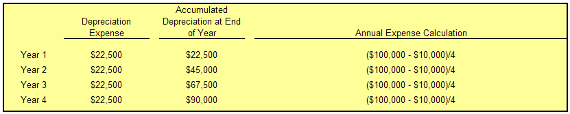
For each of the above years, the journal entry to record depreciation is as follows:
| 12-31-XX |
Depreciation Expense |
22,500 |
||
| Accumulated Depreciation |
22,500 |
|||
| To record annual depreciation expense |
The applicable depreciation expense would be included in each year's income statement (except in a manufacturing environment where some depreciation may be assigned to the manufactured inventory, as will be covered in the managerial accounting chapters later in this book). The appropriate balance sheet presentation would appear as follows (end of year 3 in this case):

FRACTIONAL PERIOD DEPRECIATION: Assets may be acquired at other than the beginning of an accounting period, and depreciation must be calculated for a partial period. With the straight-line method the amount is simply a fraction of the annual amount. For example, an asset acquired on the first day of April would be used for only nine months during the first calendar year. Therefore, year one depreciation would be 9/12 of the annual amount. Following is the depreciation table for the above asset, this time assuming an April 1 acquisition date:

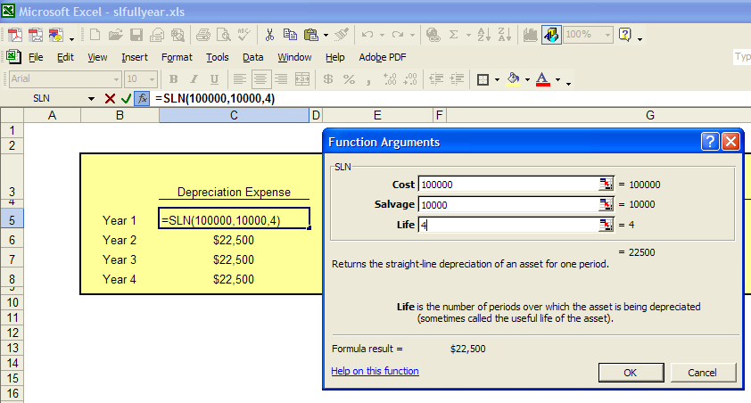
SPREADSHEET SOFTWARE: Microsoft Excel (and competing products) include built-in depreciation functions that may be entered by setting formulas (which can also be easily accessed from the Insert Function commands). Below is a screen shot showing the straight-line method function. On execution, this routine returns the $22,500 annual depreciation value to the C5 cell of the worksheet.
THE UNITS OF OUTPUT METHOD
This technique involves calculations that are quite similar to the straight-line method, but it allocates the depreciable base over the units of output (e.g., machine hours) rather than years of use. It is logical to use this approach in those situations where the life is best measured by identifiable units of machine "consumption." For example, perhaps the engine of a corporate jet has an estimated 50,000 hour life. Or, a printing machine may produce an expected 4,000,000 copies. In cases like these, the accountant may opt for the units-of-output method. To illustrate, assume Dat Nguyen Painting Corporation purchased an air filtration system that has a life of 8,000 hours. The filter costs $100,000 and has a $10,000 salvage value. Nguyen anticipates that the filter will be used 1,000 hours during the first year, 3,000 hours during the second, 2,000 during the third, and 2,000 during the fourth. Accordingly, the anticipated depreciation schedule would appear as follows (if actual usage varies, the schedule would be adjusted for the changing estimates using principles that are discussed later in this page):
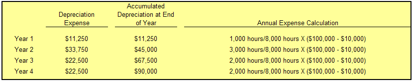
The form of journal entry and balance sheet account presentation are just as were illustrated for the straight-line method, but with the revised amounts from the above table.
THE DOUBLE-DECLINING BALANCE METHOD
As one of several "accelerated depreciation" methods, DDB results in relatively large amounts of depreciation in early years of asset life and smaller amounts in later years. This method can be justified if the quality of service produced by an asset declines over time, or if repair and maintenance costs will rise over time to offset the declining depreciation amount. With this method, a fixed percentage of the straight-line rate (i.e., 200% or "double") is multiplied times the remaining book value of an asset (as of the beginning of a particular year) to determine depreciation for a particular year. As time passes, book value and annual depreciation decrease.
To illustrate, let's again utilize our example of the $100,000 asset, with a four-year life, and $10,000 salvage value. Depreciation for each of the four years would appear as follows:
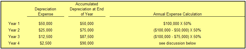
The amounts in the above table deserve additional commentary. Year one is hopefully clear -- expense equals the cost times twice the straight-line rate (4 year life = 25% straight-line rate; 25% X 2 = 50% rate). Year two is the 50% rate applied to the remaining balance of the asset as of the beginning of the year; the remaining balance would be the cost minus the accumulated depreciation ($100,000 - $50,000). Year three is just like year two -- 50% times the beginning book value ($100,000 - $75,000). Note that salvage value was simply ignored in the preliminary years' calculations. For year four, however, the calculated amount (($100,000 - $87,500) X 50% = $6,250)) would cause the lifetime depreciation to exceed the $90,000 depreciable base. Thus, in year four, only $2,500 is taken as expense even though the calculated amount is higher. This gives rise to an important general rule for DDB -- salvage value is initially ignored, but once accumulated depreciation reaches the amount of the depreciable base, then depreciation ceases. In our example, only $2,500 was needed in year four to bring the aggregate depreciation up to the $90,000 level.
It is possible that an asset will have no salvage value. If you are very perceptive, you will note that the mathematics of DDB will never fully depreciate such assets (since you are always taking only a percentage of the remaining balance, you can never bring the remaining balance to zero). In these cases, accountants typically change to the straight-line method near the end of an asset's useful life to "finish off" the accounting for an asset which is to be taken to a final zero net book value. The mechanics of this shift in method are sometimes covered in intermediate accounting.
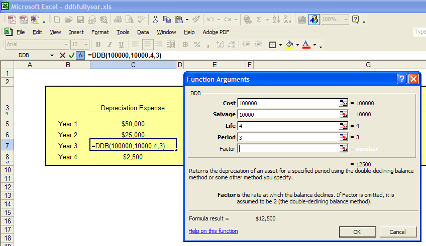
SPREADSHEET SOFTWARE: DDB is also calculable from built-in depreciation functions. Below is the routine that returns the $12,500 annual depreciation value for Year 3.
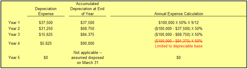
FRACTIONAL PERIOD DEPRECIATION: Under DDB, fractional years involve a very simple adaptation to the approach presented above. The first partial year will be a fraction of the annual amount, and all subsequent years will be the normal calculation (twice the straight-line rate times the beginning of year book value). If our example asset were purchased on April 1, 20X1, the following calculations result:
ALTERNATIVES TO DDB: 150% and 125% declining balance methods are quite similar to DDB, but the rate is 150% or 125% of the straight-line rate (instead of 200% as with DDB).
THE SUM-OF-THE-YEARS'-DIGITS METHOD
This approach was used in the graphic example at the beginning of this chapter, but without any calculation details. The calculations will undoubtedly be seen as a bit peculiar; I have no idea who first originated this approach or why.
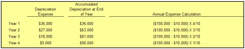
Under the technique, depreciation for any given year is determined by multiplying the depreciable base by a fraction; the numerator is a digit relating to the year of use (e.g., the digit for an asset with a ten-year life would be 10 for the first year of use, 9 for the second, and so on), and the denominator is the sum-of-the-years' digits (e.g., 10 + 9 + 8 + . . . + 2 + 1 = 55). In our continuing illustration, the four-year lived asset would be depreciated as follows (bear in mind that 4 + 3 + 2 + 1 = 10):
SPREADSHEET SOFTWARE: Again, software includes a built-in function for sum-of-the-years'-digits (SYD) method. Below is the function that returns the $18,000 annual depreciation value for Year 3.

FRACTIONAL PERIOD DEPRECIATION: With the sum-of-the-years'-digits method, fractional years require fairly intensive layering for every year (e.g., if a ten-year asset is acquired on July 1, 20X1, depreciation for 20X1 is the depreciable base times 10/55 times 6/12 (relating to six months of use); depreciation for 20X2 is the depreciable base times 10/55 times 6/12 (reflecting the last six months of the first layer), plus the depreciable base times 9/55 times 6/12 (reflecting the first six months of the next layer)). Returning to our $100,000, four-year lived asset; if the asset was acquired on April 1, Year 1, the resulting depreciation amounts are calculated as:
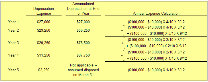
Admittedly, the above table is a bit "busy," but if you take time to trace each of the amounts, it will be a good key to your understanding.
Before moving away from the sum-of-the-years'-digits, you may find it tedious to be adding numbers like 10 + 9 + 8 + . . . + 1 = 55. But, mathematicians long ago figured out a short cut for this calculation: (n(n + 1))/2, where n is the number of items in the sequence. Thus, for an asset with a ten year life: (10 (10 + 1)/2 = 10(11)/2 = 110/2 = 55 . Try this on your own for the four year life, and make sure your result is "10." Try again for a 15 year life asset, and make sure you get "120." Do you see that the sum-of-the-years'-digit's fraction for the 4th year of use would be 12/120? Remember, you count backwards -- Year one is 15/120, Year two is 14/120, Year three is 13/120, and Year four would be 12/120.
CHANGES IN ESTIMATES: Obviously, the initial assumption about useful life and residual value is only an estimate. Time and new information may suggest that the initial assumptions need to be revised, especially if the initial estimates prove to be materially off course. It is well accepted that changes in estimates do not require re-doing the prior period financial statements; after all, an estimate is just that, and the financial statements of prior periods were presumably based on the best information available at the time. Therefore, rather than correcting prior periods' financial statements, such revisions are made prospectively (over the future) so that the remaining depreciable base is spread over the remaining life.
To illustrate, let's return to the straight-line method. Assume that two years have passed for our $100,000 asset that was initially believed to have a four-year life and $10,000 salvage value; as of the beginning of Year 3, new information suggests that the asset will have a total life of seven years (three more than originally thought), and have a $5,000 salvage value. As a result, the revised remaining depreciable base (as of January 1, 20X3) will be spread over the remaining five years, as follows:
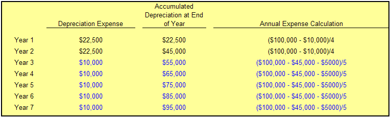
The depreciation amounts for Years 3 through 7 are based on spreading the "revised" depreciable base over the last five years of remaining life. The "revised" depreciable base is $50,000, and is calculated as the original cost ($100,000) minus the depreciation already taken ($45,000), and minus the revised salvage value ($5,000).